Setup
library(Rubrary)
library(dplyr)
#>
#> Attaching package: 'dplyr'
#> The following objects are masked from 'package:stats':
#>
#>     filter, lag
#> The following objects are masked from 'package:base':
#>
#>     intersect, setdiff, setequal, union
library(tibble)

# For `airway` install
r = getOption("repos")
r["CRAN"] = "http://cran.us.r-project.org"
options(repos = r)
Introduction
The example dataset for this vignette comes from the paper [1] below:
Himes et al. (2014). “RNA-Seq Transcriptome Profiling Identifies CRISPLD2 as a Glucocorticoid Responsive Gene that Modulates Cytokine Function in Airway Smooth Muscle Cells.” PLoS ONE, 9(6), e99625. https://doi.org/10.1371/journal.pone.0099625.
From the abstract:
Using RNA-Seq, a high-throughput sequencing method, we characterized transcriptomic changes in four primary human ASM cell lines that were treated with dexamethasone—a potent synthetic glucocorticoid (1 µM for 18 hours).
The experiment was performed on human airway smooth muscle (ASM) cells. Glucocorticoids are a commonly used drug to treat asthma for its anti-inflammatory effects in lung tissue. The goal of the experiment was to characterize the mechanism of glucocorticoid inflammation suppression through RNAseq. Himes et al. found a number of glucocorticoid-responsive genes such as DUSP1 and CRISPLD2. They also identified enrichment in functional annotation of terms such as “glycoprotein/extracellular matrix”, “vasculature development”, and “circulatory system process”.
In the original paper, the authors used Cuffdiff 2 to find differential gene expression and used the NIH Database for Annotation, Visualization, and Integrated Discovery (DAVID) for gene set enrichment analysis.
Load data
The package airway contains data from the Himes et
al. paper in the form of a RangedSummarizedExperiment object and is
hosted on Bioconductor.
Get airway data from package
if (!requireNamespace("airway", quietly = TRUE)){
  BiocManager::install("airway")
}

library(airway)
data(airway)
Get counts and sample annotation
The gene expression data is represented in counts. There are 4
samples treated with dexamethasone (anno$dex == "trt") and
4 untreated samples (anno$dex == "untrt").
# Counts
cts <- assay(airway, "counts")
# Annotation
anno <- colData(airway) %>%
  as.data.frame()
anno$dex <- relevel(anno$dex, "untrt") # Set untreated as first factor

head(cts)
#>                 SRR1039508 SRR1039509 SRR1039512 SRR1039513 SRR1039516
#> ENSG00000000003        679        448        873        408       1138
#> ENSG00000000005          0          0          0          0          0
#> ENSG00000000419        467        515        621        365        587
#> ENSG00000000457        260        211        263        164        245
#> ENSG00000000460         60         55         40         35         78
#> ENSG00000000938          0          0          2          0          1
#>                 SRR1039517 SRR1039520 SRR1039521
#> ENSG00000000003       1047        770        572
#> ENSG00000000005          0          0          0
#> ENSG00000000419        799        417        508
#> ENSG00000000457        331        233        229
#> ENSG00000000460         63         76         60
#> ENSG00000000938          0          0          0
head(anno)
#>            SampleName    cell   dex albut        Run avgLength Experiment
#> SRR1039508 GSM1275862  N61311 untrt untrt SRR1039508       126  SRX384345
#> SRR1039509 GSM1275863  N61311   trt untrt SRR1039509       126  SRX384346
#> SRR1039512 GSM1275866 N052611 untrt untrt SRR1039512       126  SRX384349
#> SRR1039513 GSM1275867 N052611   trt untrt SRR1039513        87  SRX384350
#> SRR1039516 GSM1275870 N080611 untrt untrt SRR1039516       120  SRX384353
#> SRR1039517 GSM1275871 N080611   trt untrt SRR1039517       126  SRX384354
#>               Sample    BioSample
#> SRR1039508 SRS508568 SAMN02422669
#> SRR1039509 SRS508567 SAMN02422675
#> SRR1039512 SRS508571 SAMN02422678
#> SRR1039513 SRS508572 SAMN02422670
#> SRR1039516 SRS508575 SAMN02422682
#> SRR1039517 SRS508576 SAMN02422673
DESeq2 differentially expressed genes
DESeq2 [2] performs
differential gene expression analysis my modeling counts as a negative
binomial distribution.
Create DESeqDataSet object and run DESeq
Rubrary::output_DESeq takes the DESeqResults object,
transforms it to a dataframe, and adds a sign log2 p-value column.
library(DESeq2)

dds <- DESeqDataSetFromMatrix(
  countData = cts[,rownames(anno)],
  colData = anno,
  design = ~ dex)

dds <- DESeq(dds)
#> estimating size factors
#> estimating dispersions
#> gene-wise dispersion estimates
#> mean-dispersion relationship
#> final dispersion estimates
#> fitting model and testing
res <- results(dds, contrast = c("dex", "trt", "untrt"))
deseq_res_df <- Rubrary::output_DESeq(res)
Replace Ensembl ID w/ HGNC symbol
airway gene names are given in Ensembl
ID, but HGNC
gene symbols can be easier to interpret in downstream analysis and
more compatible with gene set enrichment analysis (GSEA) tools.
# Gene format is currently in Ensembl ID format
head(deseq_res_df$gene)
#> [1] "ENSG00000152583" "ENSG00000148175" "ENSG00000179094" "ENSG00000134686"
#> [5] "ENSG00000125148" "ENSG00000120129"

library(biomaRt)
#> Warning: replacing previous import 'utils::findMatches' by
#> 'S4Vectors::findMatches' when loading 'AnnotationDbi'
# Load Mart object - database of Homo sapiens genes from Ensembl
mart <- biomaRt::useDataset(
  dataset = "hsapiens_gene_ensembl",
  mart = biomaRt::useMart("ENSEMBL_MART_ENSEMBL"))

conv <- Rubrary::convert_genes(
    genes = deseq_res_df$gene,
    from_to = c("ensembl_gene_id", "hgnc_symbol"),
    mart = mart, table = T) %>%
  filter(hgnc_symbol != "") %>% # Exclude unmatched HGNC symbols
  distinct(hgnc_symbol, .keep_all = T)

deseq_res_hgnc <- dplyr::left_join( # Join stats with HGNC symbol table
  conv, deseq_res_df, by = join_by(ensembl_gene_id == gene)) %>%
  arrange(desc(sign_log_p))

# Genes now have associated HGNC symbols
head(deseq_res_hgnc)
#>   ensembl_gene_id hgnc_symbol   baseMean log2FoldChange      lfcSE     stat
#> 1 ENSG00000152583     SPARCL1   997.4398       4.602526 0.21177076 21.73353
#> 2 ENSG00000148175        STOM 11193.7188       1.451466 0.08482489 17.11132
#> 3 ENSG00000179094        PER1   776.5967       3.183858 0.20151544 15.79957
#> 4 ENSG00000134686        PHC2  2737.9820       1.387141 0.09158425 15.14607
#> 5 ENSG00000125148        MT2A  3656.2528       2.203439 0.14740866 14.94782
#> 6 ENSG00000120129       DUSP1  3409.0294       2.948984 0.20161362 14.62691
#>          pvalue          padj sign_log_p
#> 1 9.889991e-105 1.838055e-100   345.4965
#> 2  1.221959e-65  1.135505e-61   215.6361
#> 3  3.132381e-56  1.940510e-52   184.3807
#> 4  8.043913e-52  3.737403e-48   169.7324
#> 5  1.609198e-50  5.981389e-47   165.4101
#> 6  1.891923e-48  5.860231e-45   158.5327
Filter to protein coding genes
For ease of interpretation, the DE genes results can also be filtered
to protein coding genes only. Rubrary::filter_genes() can
filter with the list of protein coding genes retrieved with
Rubrary::get_PC_genes(). Since we already created the
Mart object when converting gene symbols, we can reuse it
to avoid querying the BioMart database again and load protein coding
genes efficiently.
deseq_res_hgnc_PC <- Rubrary::filter_genes(
df = deseq_res_hgnc,
gene_col = "hgnc_symbol",
genes_filt = Rubrary::get_PC_genes(mart)
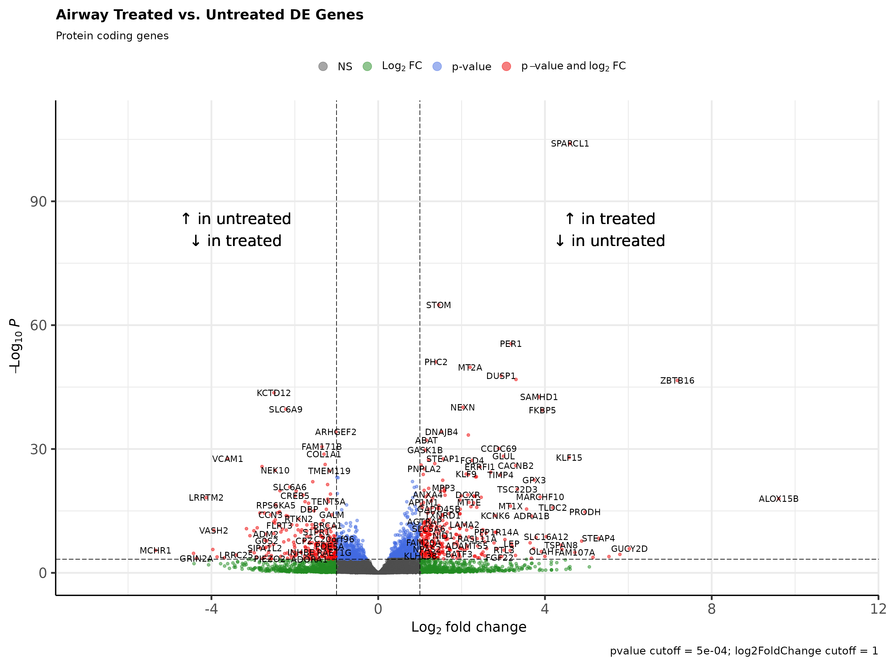
)Volcano plot
DESeq results can be visualized through volcano plots. Volcano plots show that top and bottom differentially expressed genes when sorted by decreasing signed log p value present as outliers on the top right and top left.
# All DE genes
head(deseq_res_hgnc[order(deseq_res_hgnc$sign_log_p, decreasing = T),])
#>   ensembl_gene_id hgnc_symbol   baseMean log2FoldChange      lfcSE     stat
#> 1 ENSG00000152583     SPARCL1   997.4398       4.602526 0.21177076 21.73353
#> 2 ENSG00000148175        STOM 11193.7188       1.451466 0.08482489 17.11132
#> 3 ENSG00000179094        PER1   776.5967       3.183858 0.20151544 15.79957
#> 4 ENSG00000134686        PHC2  2737.9820       1.387141 0.09158425 15.14607
#> 5 ENSG00000125148        MT2A  3656.2528       2.203439 0.14740866 14.94782
#> 6 ENSG00000120129       DUSP1  3409.0294       2.948984 0.20161362 14.62691
#>          pvalue          padj sign_log_p
#> 1 9.889991e-105 1.838055e-100   345.4965
#> 2  1.221959e-65  1.135505e-61   215.6361
#> 3  3.132381e-56  1.940510e-52   184.3807
#> 4  8.043913e-52  3.737403e-48   169.7324
#> 5  1.609198e-50  5.981389e-47   165.4101
#> 6  1.891923e-48  5.860231e-45   158.5327
tail(deseq_res_hgnc[order(deseq_res_hgnc$sign_log_p, decreasing = T),])
#>       ensembl_gene_id hgnc_symbol    baseMean log2FoldChange      lfcSE
#> 25081 ENSG00000162692       VCAM1    508.1702      -3.609367 0.32654691
#> 25082 ENSG00000108821      COL1A1 100990.6944      -1.299499 0.11528151
#> 25083 ENSG00000144369     FAM171B   1303.2727      -1.350324 0.11607419
#> 25084 ENSG00000116584     ARHGEF2   2250.5969      -1.014517 0.08232161
#> 25085 ENSG00000196517      SLC6A9    229.6407      -2.216934 0.16666134
#> 25086 ENSG00000178695      KCTD12   2649.8501      -2.499912 0.17893290
#>            stat       pvalue         padj sign_log_p
#> 25081 -11.05314 2.116887e-28 1.639264e-25  -91.93204
#> 25082 -11.27239 1.796180e-29 1.589619e-26  -95.49098
#> 25083 -11.63328 2.791614e-31 2.882341e-28 -101.49867
#> 25084 -12.32382 6.742097e-35 8.353458e-32 -113.51429
#> 25085 -13.30203 2.252620e-40 3.488745e-37 -131.70552
#> 25086 -13.97123 2.335645e-44 4.823106e-41 -144.94102

Rubrary::plot_volcano(
  df_deg = deseq_res_hgnc,
  names = "hgnc_symbol",
  x = "log2FoldChange", y = "pvalue",
  FCcutoff = 1, pCutoff = 5e-04,
  title = "Airway Treated vs. Untreated DE Genes",
  xlab_high = "\U2191 in treated,\n\U2193 in untreated",
  xlab_low = "\U2191 in untreated,\n\U2193 in treated",
  subtitle = "All genes"
)
# Protein coding DE genes
head(deseq_res_hgnc_PC[order(deseq_res_hgnc$sign_log_p, decreasing = T),])
#>   ensembl_gene_id hgnc_symbol   baseMean log2FoldChange      lfcSE     stat
#> 1 ENSG00000152583     SPARCL1   997.4398       4.602526 0.21177076 21.73353
#> 2 ENSG00000148175        STOM 11193.7188       1.451466 0.08482489 17.11132
#> 3 ENSG00000179094        PER1   776.5967       3.183858 0.20151544 15.79957
#> 4 ENSG00000134686        PHC2  2737.9820       1.387141 0.09158425 15.14607
#> 5 ENSG00000125148        MT2A  3656.2528       2.203439 0.14740866 14.94782
#> 6 ENSG00000120129       DUSP1  3409.0294       2.948984 0.20161362 14.62691
#>          pvalue          padj sign_log_p
#> 1 9.889991e-105 1.838055e-100   345.4965
#> 2  1.221959e-65  1.135505e-61   215.6361
#> 3  3.132381e-56  1.940510e-52   184.3807
#> 4  8.043913e-52  3.737403e-48   169.7324
#> 5  1.609198e-50  5.981389e-47   165.4101
#> 6  1.891923e-48  5.860231e-45   158.5327
tail(deseq_res_hgnc_PC[order(deseq_res_hgnc$sign_log_p, decreasing = T),])
#>         ensembl_gene_id hgnc_symbol baseMean log2FoldChange lfcSE stat pvalue
#> NA.8620            <NA>        <NA>       NA             NA    NA   NA     NA
#> NA.8621            <NA>        <NA>       NA             NA    NA   NA     NA
#> NA.8622            <NA>        <NA>       NA             NA    NA   NA     NA
#> NA.8623            <NA>        <NA>       NA             NA    NA   NA     NA
#> NA.8624            <NA>        <NA>       NA             NA    NA   NA     NA
#> NA.8625            <NA>        <NA>       NA             NA    NA   NA     NA
#>         padj sign_log_p
#> NA.8620   NA         NA
#> NA.8621   NA         NA
#> NA.8622   NA         NA
#> NA.8623   NA         NA
#> NA.8624   NA         NA
#> NA.8625   NA         NA

Rubrary::plot_volcano(
  df_deg = deseq_res_hgnc_PC,
  names = "hgnc_symbol",
  x = "log2FoldChange", y = "pvalue",
  FCcutoff = 1, pCutoff = 5e-04,
  title = "Airway Treated vs. Untreated DE Genes",
  xlab_high = "\U2191 in treated\n\U2193 in untreated",
  xlab_low = "\U2191 in untreated\n\U2193 in treated",
  subtitle = "Protein coding genes"
)
fgsea gene set enrichment analysis
fgsea [3] is an
implementation of an algorithm for fast gene set enrichment analysis
(GSEA), based on the original GSEA algorithm [4].
Get pathways from msigdbr
Gene set enrichment analysis relies on inputting gene sets / pathways
related to biological function. The Molecular Signatures Database
(MSigDB) [5] was published as a database
of annotated pathways to facilitate GSEA and is accessible through the R
package msigdbr [6].
C2CP: curated gene sets, canonical pathways
-
C5GO: ontology gene sets, Gene Ontology gene sets
BP: GO Biological Process ontology
CC: GO Cellular Component ontology
MF: GO Molecular Function ontology
H: hallmark gene sets [7]
if (!requireNamespace("msigdbr", quietly = TRUE)){
  BiocManager::install("msigdbr")
}

msigdbr::msigdbr_collections()
#> # A tibble: 23 × 3
#>    gs_cat gs_subcat         num_genesets
#>    <chr>  <chr>                    <int>
#>  1 C1     ""                         299
#>  2 C2     "CGP"                     3384
#>  3 C2     "CP"                        29
#>  4 C2     "CP:BIOCARTA"              292
#>  5 C2     "CP:KEGG"                  186
#>  6 C2     "CP:PID"                   196
#>  7 C2     "CP:REACTOME"             1615
#>  8 C2     "CP:WIKIPATHWAYS"          664
#>  9 C3     "MIR:MIRDB"               2377
#> 10 C3     "MIR:MIR_Legacy"           221
#> # ℹ 13 more rows

pthwys <- rbind(
  msigdbr::msigdbr(category = "C2", subcategory = "CP"),
  msigdbr::msigdbr(category = "C5", subcategory = "GO:BP"),
  msigdbr::msigdbr(category = "C5", subcategory = "GO:CC"),
  msigdbr::msigdbr(category = "C5", subcategory = "GO:MF"),
  msigdbr::msigdbr(category = "H")
) %>%
  split(x = .$gene_symbol, f = .$gs_name) # Named list of pathways
Run fgsea
# `fgsea` requires a named numeric vector as input to the `stats` argument
deseq_stats <- setNames(
    deseq_res_hgnc_PC[,"sign_log_p"],
    deseq_res_hgnc_PC[,"hgnc_symbol"]
)

gsea_results <- fgsea::fgsea(
  pathways = pthwys,
  stats = deseq_stats,
  eps = 0.0,
  minSize = 15,
  maxSize  = 500) %>%
  arrange(desc(NES)) %>%
  mutate(sign_log10_p = sign(NES) * -log10(pval)) # Create sign_log10_p column
#> Warning in preparePathwaysAndStats(pathways, stats, minSize, maxSize, gseaParam, : There are ties in the preranked stats (6.92% of the list).
#> The order of those tied genes will be arbitrary, which may produce unexpected results.
Visualize GSEA results as a table
See the GSEA User Guide: Interpreting GSEA Results for detailed explanation in interpreting results.
# Get top significant pathways by positive/negative enrichment score (ES)
pos_pws <- gsea_results[ES > 0][head(order(pval), n = 5), pathway]
neg_pws <- gsea_results[ES < 0][head(order(pval), n = 5), pathway]
top_pws <- c(pos_pws, rev(neg_pws))

fgsea::plotGseaTable(
  pathways = pthwys[top_pws],
  stats = deseq_stats,
  fgseaRes = gsea_results,
  gseaParam = 0.5
)
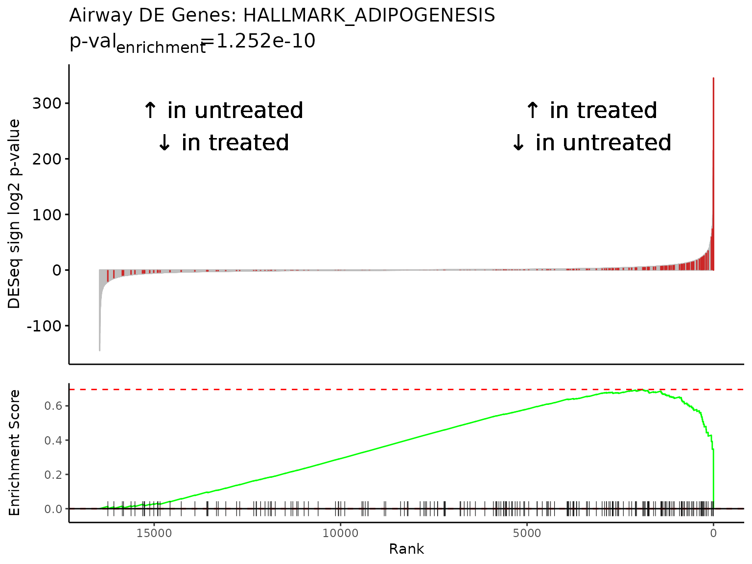
Pathway enrichment plot
Specific pathways of interest can be plotted in GSEA Java app-like enrichment plots that combine a waterfall and mountain plot.
The top enriched pathway from our GSEA results is “HALLMARK_ADIPOGENESIS”, a collection of 196 genes up-regulated during adipocyte (fat cell) differentiation. This is in line with studies reporting the complex effects of glucocorticoids on adipose tissue biology, including differentiation of adipocyte precursors and adipogenesis [8,9].
The maximum absolute value in the Enrichment Score mountain plot
corresponds to the ES value reported in the GSEA
results.
gsea_results[gsea_results$pathway == "HALLMARK_ADIPOGENESIS",]
#>                  pathway         pval         padj   log2err        ES      NES
#> 1: HALLMARK_ADIPOGENESIS 4.336231e-07 0.0007532034 0.6749629 0.6955378 1.905522
#>    size                           leadingEdge sign_log10_p
#> 1:  196 SPARCL1,STOM,GPX3,TST,SLC5A6,SQOR,...     6.362888

Rubrary::plot_GSEA_pathway(
  sig = deseq_res_hgnc_PC,
  geneset = pthwys[["HALLMARK_ADIPOGENESIS"]],
  genecol = "hgnc_symbol",
  rankcol = "sign_log_p",
  rankcol_name = "DESeq sign log2 p-value",
  label = FALSE,
  title = "Airway DE Genes: HALLMARK_ADIPOGENESIS",
  lab_high = "\U2191 in treated\n\U2193 in untreated",
  lab_low = "\U2191 in untreated\n\U2193 in treated"
)
For gene sets of smaller sizes, like 20 gene pathway “GOBP_NEURON_FATE_SPECIFICATION”, labeling each gene may be appropriate.
gsea_results[gsea_results$pathway == "GOBP_NEURON_FATE_SPECIFICATION",]
#>                           pathway         pval       padj   log2err         ES
#> 1: GOBP_NEURON_FATE_SPECIFICATION 0.0002154196 0.08538821 0.5188481 -0.8621391
#>          NES size               leadingEdge sign_log10_p
#> 1: -1.835486   20 GLI2,SUFU,GLI3,EYA1,EHMT2    -3.666715

Rubrary::plot_GSEA_pathway(
  sig = deseq_res_hgnc_PC,
  geneset = pthwys[["GOBP_NEURON_FATE_SPECIFICATION"]],
  genecol = "hgnc_symbol",
  rankcol = "sign_log_p",
  rankcol_name = "DESeq sign log2 p-value",
  label = TRUE,
  title = "Airway DE Genes: GOBP_NEURON_FATE_SPECIFICATION",
  lab_high = "\U2191 in treated\n\U2193 in untreated",
  lab_low = "\U2191 in untreated\n\U2193 in treated"
)
#> Warning: Removed 16440 rows containing missing values
#> (`geom_text_repel()`).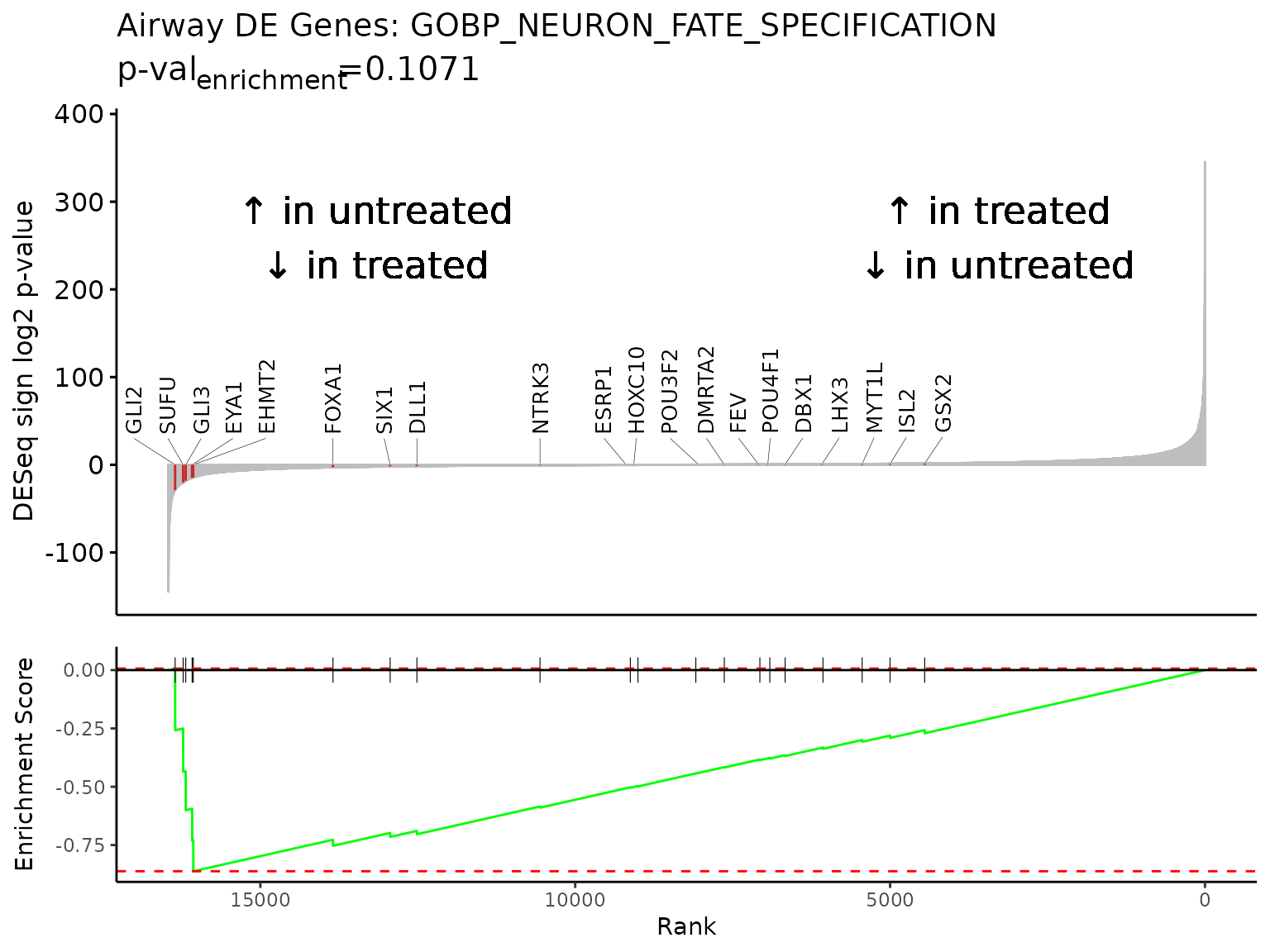
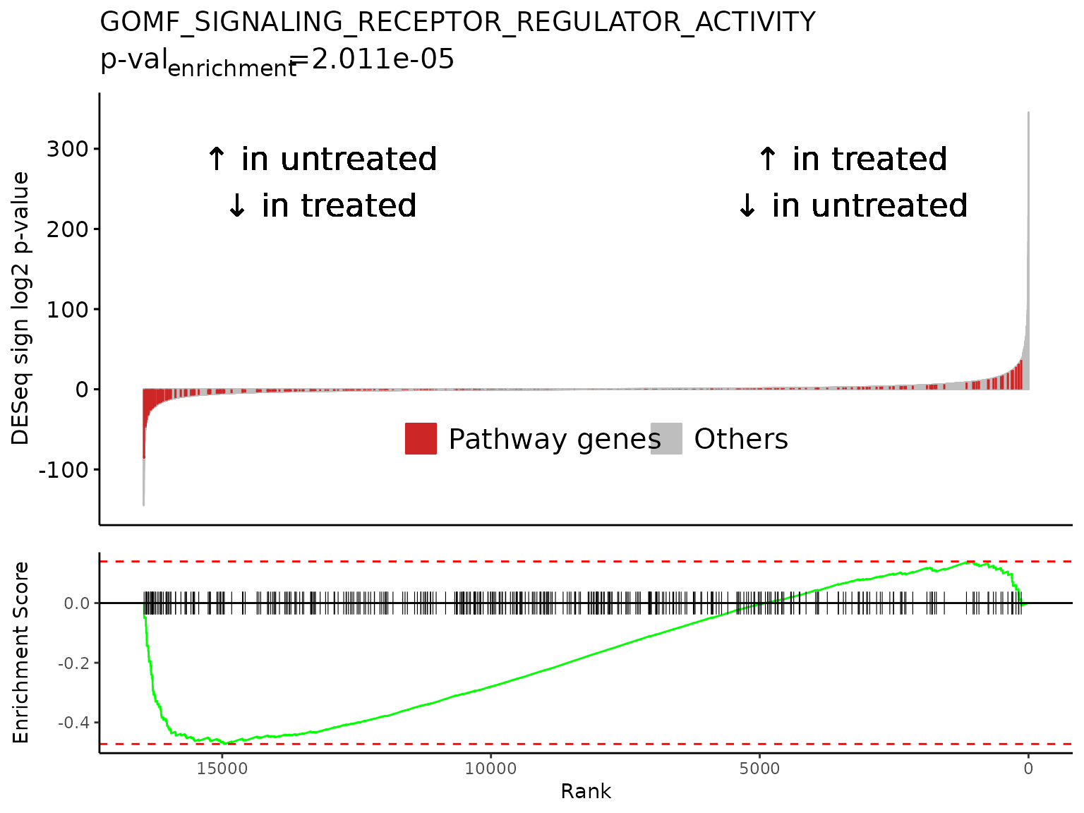
Multiple gene set enrichment plots can be created in a batch with
Rubrary::plot_GSEA_batch, a wrapper for
Rubrary::plot_GSEA_pathway that works well with
lapply. We can use the neg_pws list of pathway
names to plot gene enrichment plots for the most significant negatively
enriched pathways.
gsea_results[gsea_results$pathway %in% neg_pws,]
#>                                          pathway         pval         padj
#> 1:    GOMF_SIGNALING_RECEPTOR_REGULATOR_ACTIVITY 4.261417e-06 0.0055515605
#> 2:                        GOCC_SYNAPTIC_MEMBRANE 4.074127e-07 0.0007532034
#> 3:                     GOCC_PRESYNAPTIC_MEMBRANE 1.878609e-05 0.0163157167
#> 4: GOCC_INTRINSIC_COMPONENT_OF_SYNAPTIC_MEMBRANE 1.749676e-05 0.0163157167
#> 5:                    GOCC_POSTSYNAPTIC_MEMBRANE 8.500710e-08 0.0004429720
#>      log2err         ES       NES size
#> 1: 0.6105269 -0.4721901 -1.625213  387
#> 2: 0.6749629 -0.5283197 -1.774112  319
#> 3: 0.5756103 -0.6039770 -1.832044  127
#> 4: 0.5756103 -0.6182693 -1.881121  128
#> 5: 0.7049757 -0.5817831 -1.884854  226
#>                                    leadingEdge sign_log10_p
#> 1:        TSLP,CCN3,LIF,CXCL12,FLRT3,GDF15,...    -5.370446
#> 2:  KCTD12,SLC6A9,SLC6A6,LRRTM2,DNM1,FLRT3,...    -6.389965
#> 3:  KCTD12,SLC6A9,DNM1,ADCY8,EPHB2,NECTIN1,...    -4.726164
#> 4:  SLC6A9,SLC6A6,LRRTM2,FLRT3,ADCY8,EPHB2,...    -4.757042
#> 5: KCTD12,SLC6A9,SLC6A6,LRRTM2,FLRT3,CNIH3,...    -7.070545

lapply(
  neg_pws[1:3],
  FUN = Rubrary::plot_GSEA_batch,
  genecol = "hgnc_symbol",
  pthwys = pthwys,
  sig = deseq_res_hgnc_PC,
  rankcol = "sign_log_p",
  rankcol_name = "DESeq sign log2 p-value",
  hllab = "Pathway genes",
  lab_high = "\U2191 in treated\n\U2193 in untreated",
  lab_low = "\U2191 in untreated\n\U2193 in treated"
)
#> [[1]]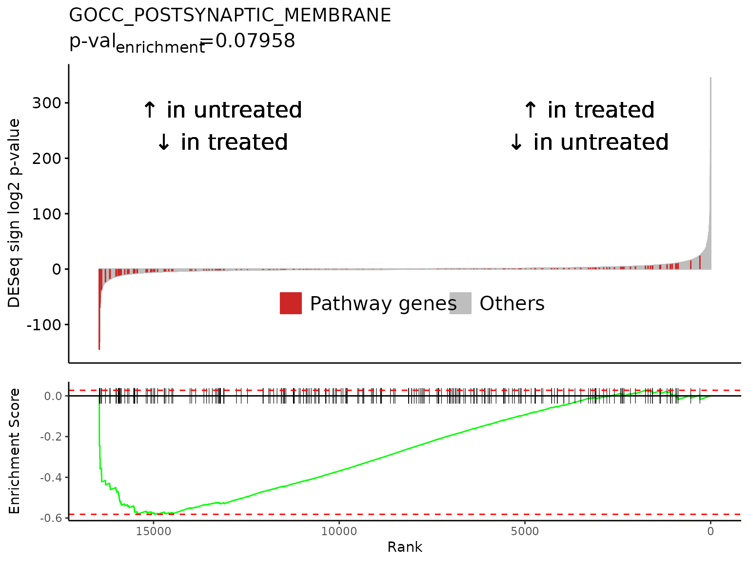
#>
#> [[2]]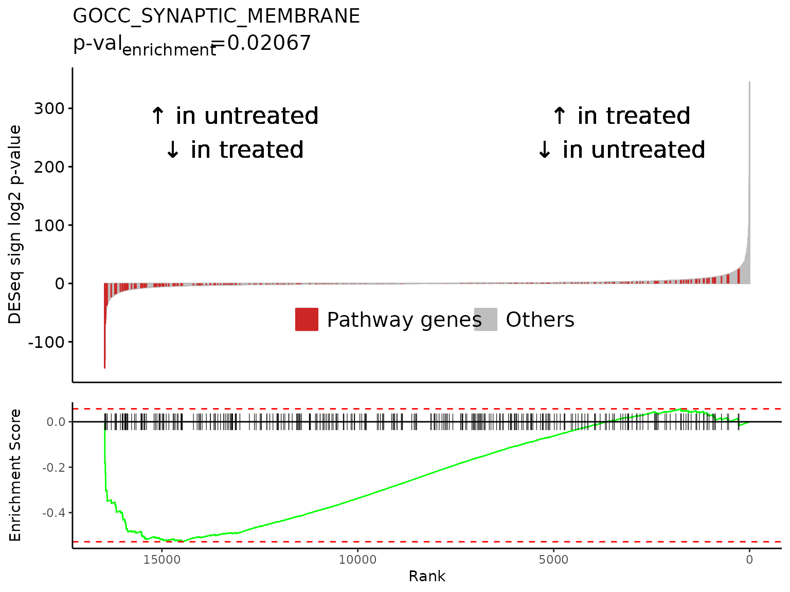
#>
#> [[3]]