Plot PCA with annotation

Usage

plot_PCA(
  df_pca,
  anno = NULL,
  PCx = "PC1",
  PCy = "PC2",
  type = c("Scores", "Loadings"),
  annoname = "Sample",
  annolabel = annoname,
  label = FALSE,
  annotype = "Type",
  annotype2 = NULL,
  ellipse = FALSE,
  ks_pval = c("none", "caption", "grob"),
  highlight = NULL,
  colors = NULL,
  col_midpt = 0,
  title = NULL,
  subtitle = NULL,
  density = FALSE,
  savename = NULL,
  width = 8,
  height = 8
)

Arguments

df_pca: string or prcomp obj; (path to) PCA output
anno: string or df; Annotation info for DF
PCx: string; Component on x-axis
PCy: string; Component on y-axis
type: c("Score", "Loading")
annoname: string; Colname in anno matching point name
annolabel: string; Colname in anno to label points by, defaults to annoname
label: logical; T to label points
annotype: string; Colname in anno with info to color by
annotype2: string; Colname in anno with info to change shape by
ellipse: logical; Draw ggplot2::stat_ellipse data ellipse w/ default params - this is NOT a confidence ellipse
ks_pval: c("none", "caption", "grob"); Display ks-pvalue as caption or grob
highlight: char vector; Specific points to shape differently & label
colors: char vector; For discrete annotype, length should be number of unique annotypes. For continuous annotype, can either be length 2 where colors[1] is low and colors[2] is high or length 3 diverging colorscale where colors[1] = low, colors[2] = mid, colors[3] = high.
col_midpt: numeric; For continuous length(colors) == 3 scale_color_gradientn usage only
title: string; Plot title
subtitle: string; Subtitle for plot
density: logical; Show density plot along both axes; requires group annotations to be provided
savename: string; File path to save plot under
width: numeric; Saved plot width
height: numeric; Saved plot height

Value

PCA output plotted with annotation

Examples

data(iris)
iris$Sample = rownames(iris)
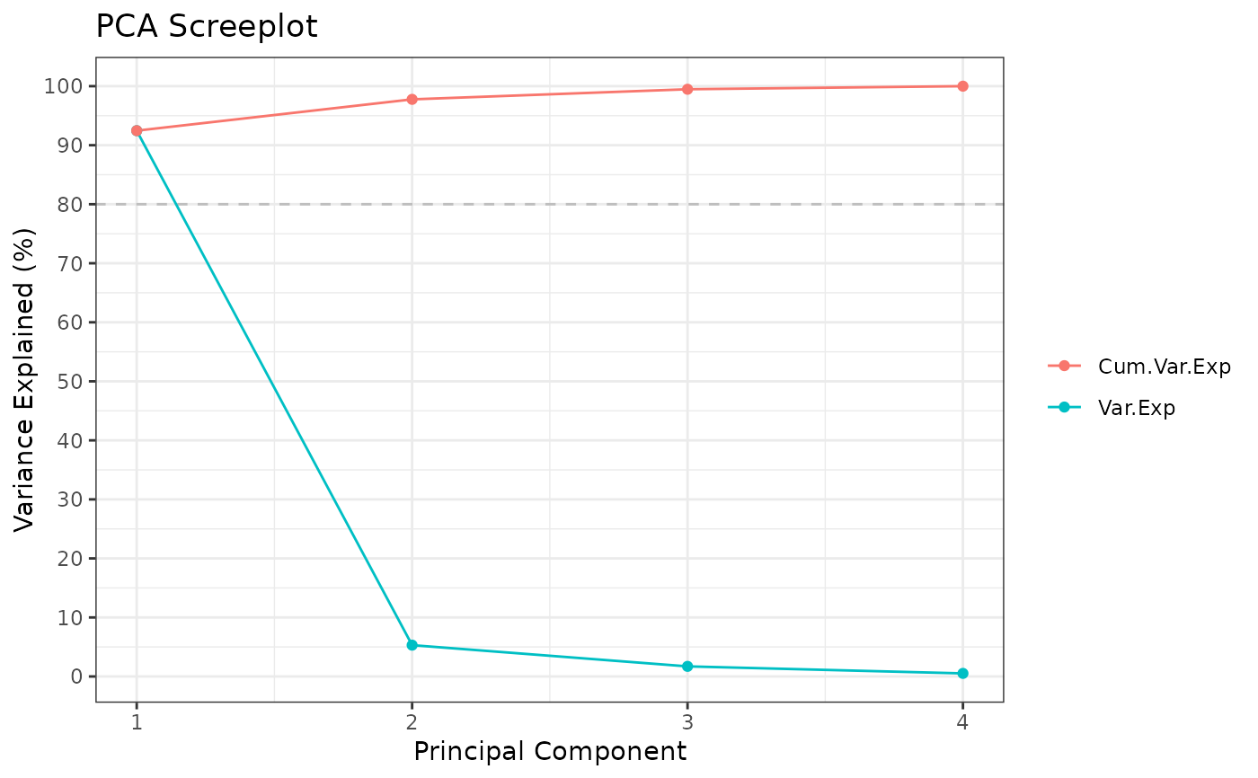
PCA_iris <- Rubrary::run_PCA(t(iris[,c(1:4)]))
#> ** Cumulative var. exp. >= 80% at PC 1 (92.5%)

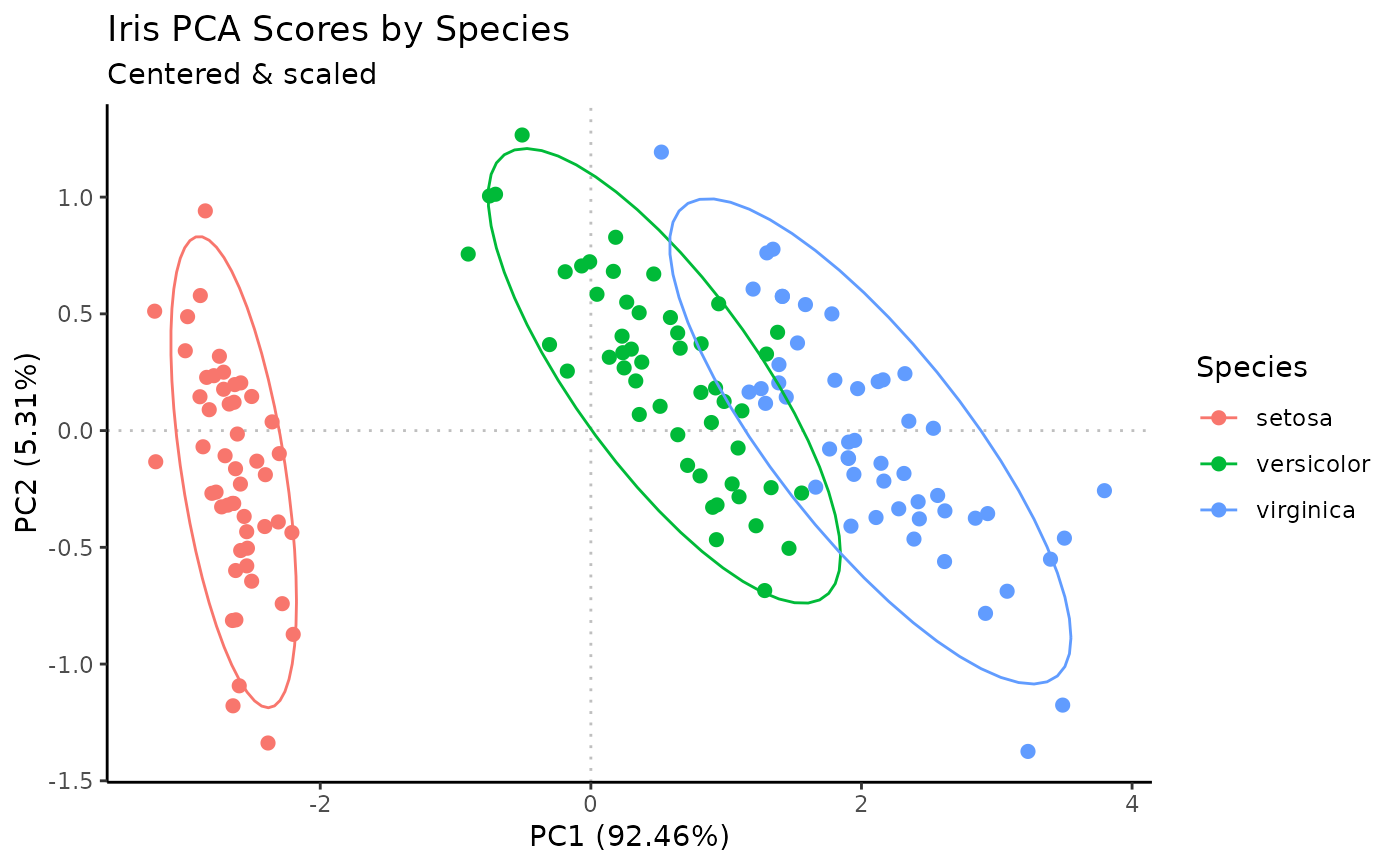
# Scores
Rubrary::plot_PCA(
  df_pca = PCA_iris,
  anno = iris[,c("Sample", "Species")],
  annoname = "Sample", annotype = "Species",
  title = "Iris PCA Scores by Species",
  subtitle = "Centered & scaled",
  ellipse = TRUE
)

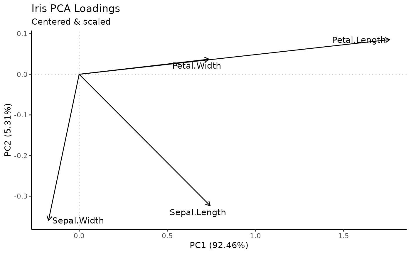
# Loadings
Rubrary::plot_PCA(
  df_pca = PCA_iris,
  type = "Loadings",
  title = "Iris PCA Loadings",
  subtitle = "Centered & scaled",
  label = TRUE
)