Principal Component Analysis (PCA) Quickstart

Yi Jou (Ruby) Liao

library(Rubrary)
library(dplyr)

# For `palmerpenguins` install
r = getOption("repos")
r["CRAN"] = "http://cran.us.r-project.org"
options(repos = r)

This vignette goes over how to run the PCA related functions in Rubrary for dimensional reduction and visualization. For a more math-y, in-depth step by step walkthrough with lengthier explanations see the PCA Walkthrough vignette.

Beltran et al. 2016 PCA

This replicates the PCA portions of the graeberlab-ucla/glab.library PCA tutorial using Beltran et al. 2016(Beltran et al. 2016) CRPC/NEPC data that initiate many new computational Graeber Lab members into the lab.

Load data

Raw text files can be loaded through read.delim by passing in the URL.

# Upper quartile normalized log2 transformed gene counts
Beltran_log2UQ_exp <- Rubrary::rread("https://raw.githubusercontent.com/graeberlab-ucla/glab.library/master/vignettes/PCA_tutorial/Beltran_2016_rsem_genes_upper_norm_counts_coding_log2.txt", row.names = 1)

rmarkdown::paged_table(Rubrary::corner(Beltran_log2UQ_exp))

Run PCA

Generally, scaling is unnecessary for log transformed gene expression because all features (genes) have the same unit of measure and it is assumed that scales are relatively similar across all genes.

Centering should always be performed for PCA to result in maximizing variance.

See the Standardization section in the PCA Walkthrough for more info.

Beltran_PCA <- Rubrary::run_PCA(
  df = Beltran_log2UQ_exp,
  center = TRUE, scale = FALSE
)
#> ** Cumulative var. exp. >= 80% at PC 18 (80.5%)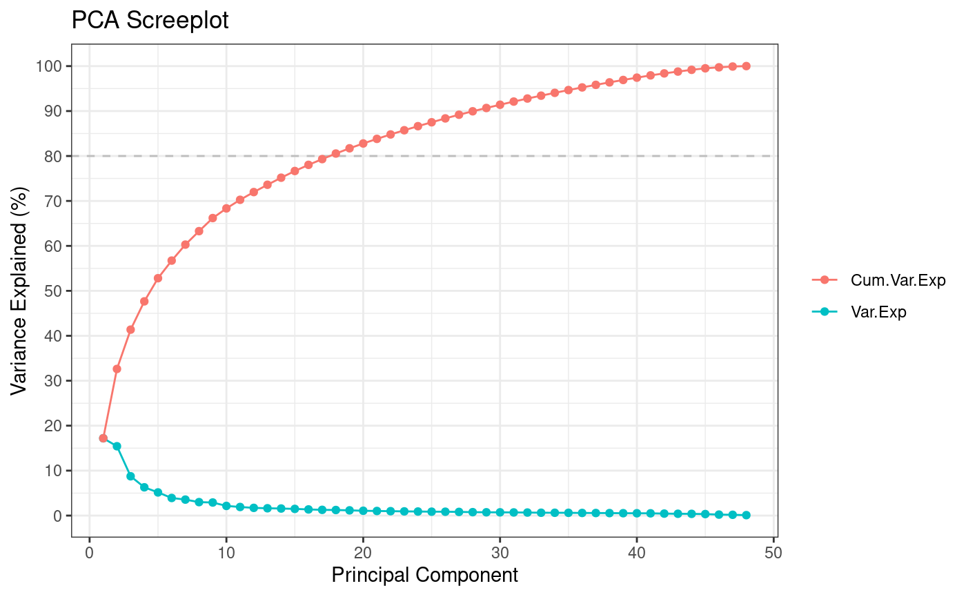

Plot PCA

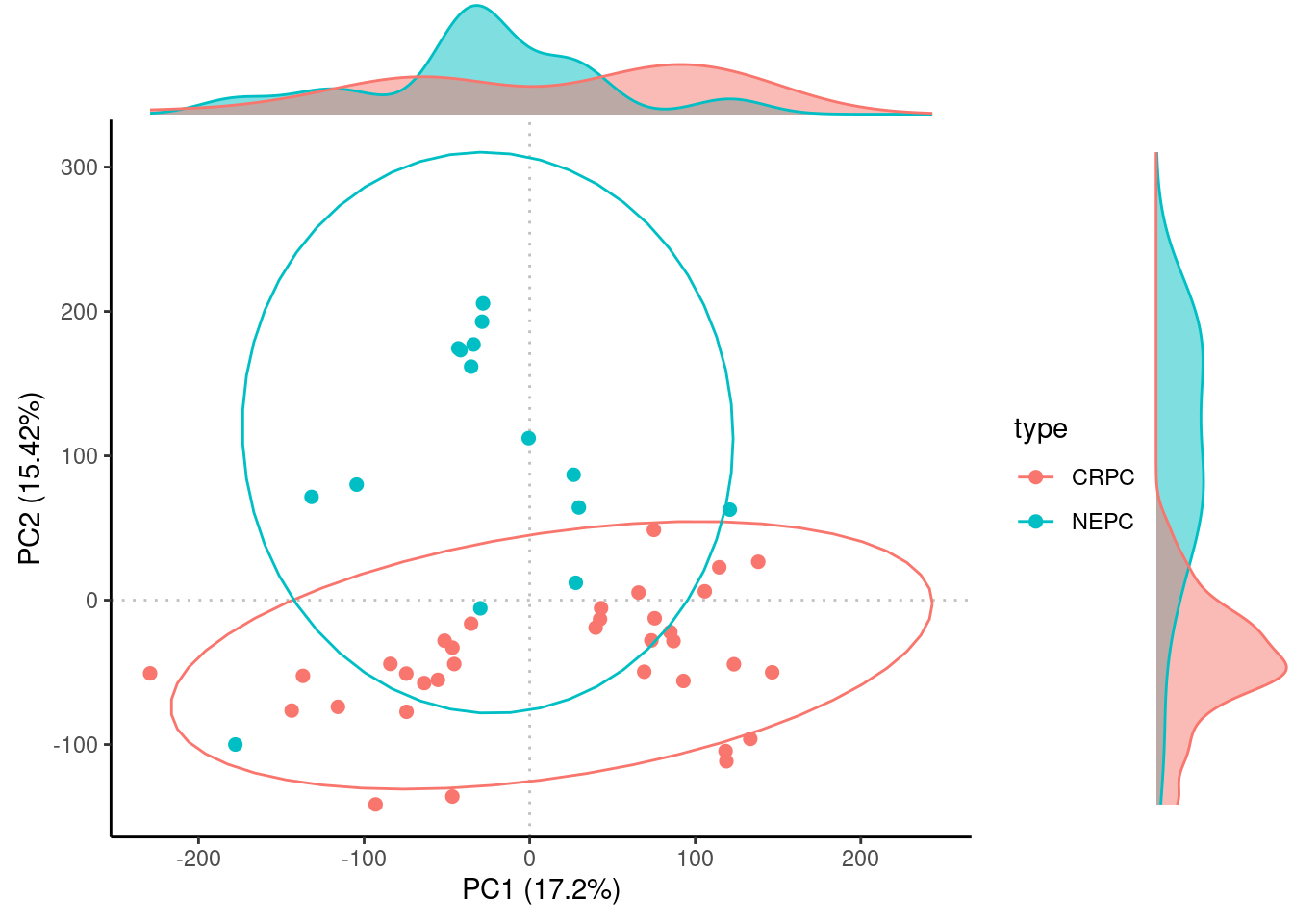
The annotations are in a huge file associating a large number of samples with its cancer type abbreviation. In this dataset, the samples correspond to “CRPC”, castration resistant prostate cancer, and “NEPC”, neuroendocrine prostate cancer.

# Annotation file
Beltran_info <- read.delim("https://raw.githubusercontent.com/graeberlab-ucla/glab.library/master/vignettes/PCA_tutorial/human.info.rsem.expression.txt")

head(Beltran_info)
#>            sample type
#> 1 TCGA.05.4244.01 LUAD
#> 2 TCGA.05.4249.01 LUAD
#> 3 TCGA.05.4250.01 LUAD
#> 4 TCGA.05.4382.01 LUAD
#> 5 TCGA.05.4384.01 LUAD
#> 6 TCGA.05.4389.01 LUAD

The NEPC and CRPC samples separate pretty nicely along PC2.

Rubrary::plot_PCA(
  df_pca = Beltran_PCA,
  type = "Scores",
  anno = Beltran_info,
  annoname = "sample",
  annotype = "type",
  density = T, ellipse = T
)

Lower PCs can be visualized simultaneously with Rubrary::plot_PCA_matrix.

Rubrary::plot_PCA_matrix(
  df_pca = Beltran_PCA,
  PCs = c(1:5),
  anno = Beltran_info,
  annoname = "sample",
  annotype = "type"
)
#> Registered S3 method overwritten by 'GGally':
#>   method from   
#>   +.gg   ggplot2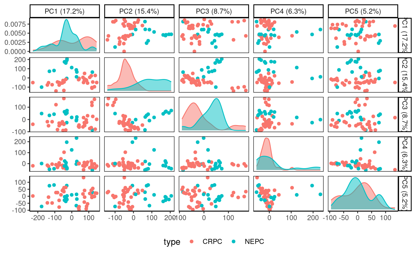

3D view of the first three PCs.

Rubrary::plot_PCA_3D(
  df_pca = Beltran_PCA,
  PCs = c(1:3),
  anno = Beltran_info,
  annoname = "sample",
  annotype = "type"
)

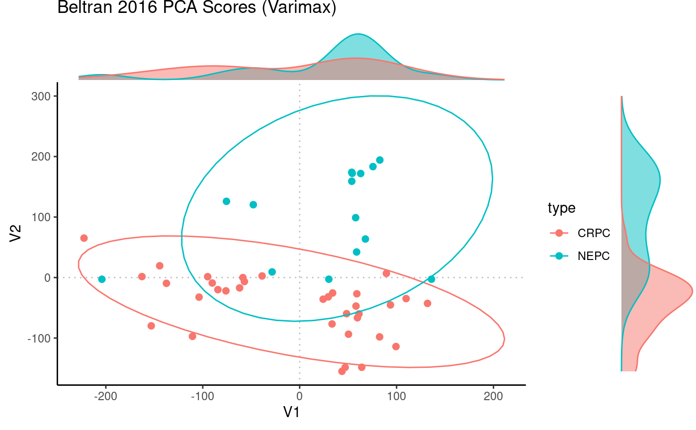
Varimax rotation

Beltran_PCA_VM <- Rubrary::rotate_varimax(Beltran_PCA, normalize = FALSE)

# Visualize scores
Rubrary::plot_PCA(
  df_pca = Beltran_PCA_VM$scores,
  PCx = "V1", PCy = "V2",
  title = "Beltran 2016 PCA Scores (Varimax)",
  type = "Scores",
  anno = Beltran_info,
  annoname = "sample",
  annotype = "type",
  density = T, ellipse = T
)

Palmer Penguins PCA

Using palmerpenguins dataset from Allison Horst.

Load data

Get palmerpenguins data and add a unique ID per entry.

if (!requireNamespace("palmerpenguins", quietly = TRUE)){
  install.packages("palmerpenguins")
}
library(palmerpenguins)

penguins <- penguins %>%
  as.data.frame() %>%
  mutate(Sample_ID = paste0(penguins_raw$`Individual ID`, "_", penguins_raw$`Sample Number`))
  
rownames(penguins) <- penguins$Sample_ID

rmarkdown::paged_table(penguins)

Run PCA

Subset data to numeric only, then run PCA.

num <- penguins %>%
  dplyr::select(!c(species, island, sex, year, Sample_ID)) %>%
  t() %>%
  as.data.frame() %>%
  dplyr::select(where(~!all(is.na(.x)))) # Filter out NAs
  
pca <- Rubrary::run_PCA(
  df = num,
  summary = T, tol = 0,
  center = T, scale = T,
  screeplot = T
)
#> ** Cumulative var. exp. >= 80% at PC 2 (88.2%)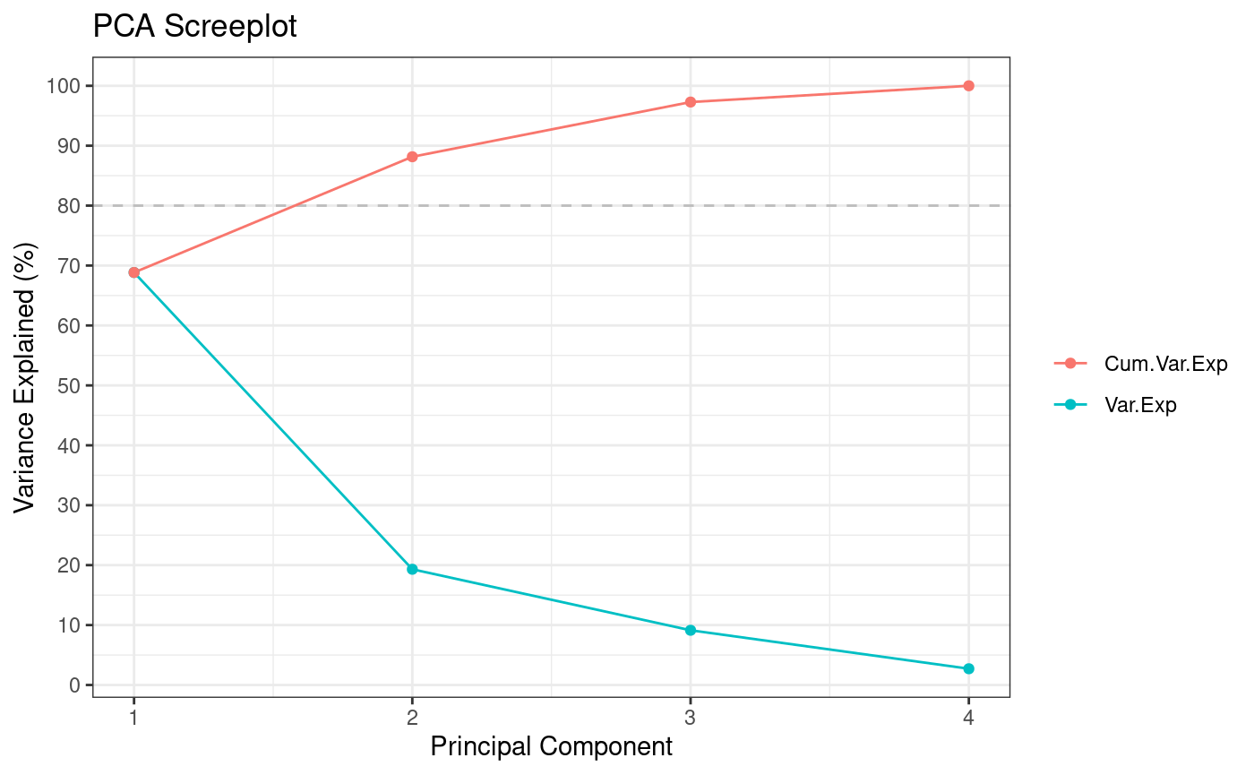

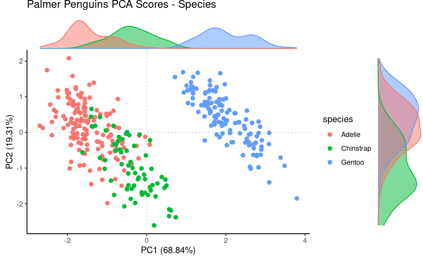
Plot PCA

Use resulting prcomp object to plot PCA scores while annotating by species metadata.

Rubrary::plot_PCA(
  df_pca = pca,
  anno = penguins,
  annoname = "Sample_ID",
  annotype = "species",
  title = "Palmer Penguins PCA Scores - Species",
  label = FALSE,
  density = TRUE
)

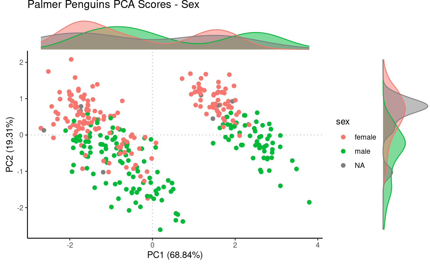
Same PCA scores plot, but annotating by sex metadata.

Rubrary::plot_PCA(
  df_pca = pca,
  anno = penguins,
  annoname = "Sample_ID",
  annotype = "sex",
  title = "Palmer Penguins PCA Scores - Sex",
  label = FALSE,
  density = TRUE
)

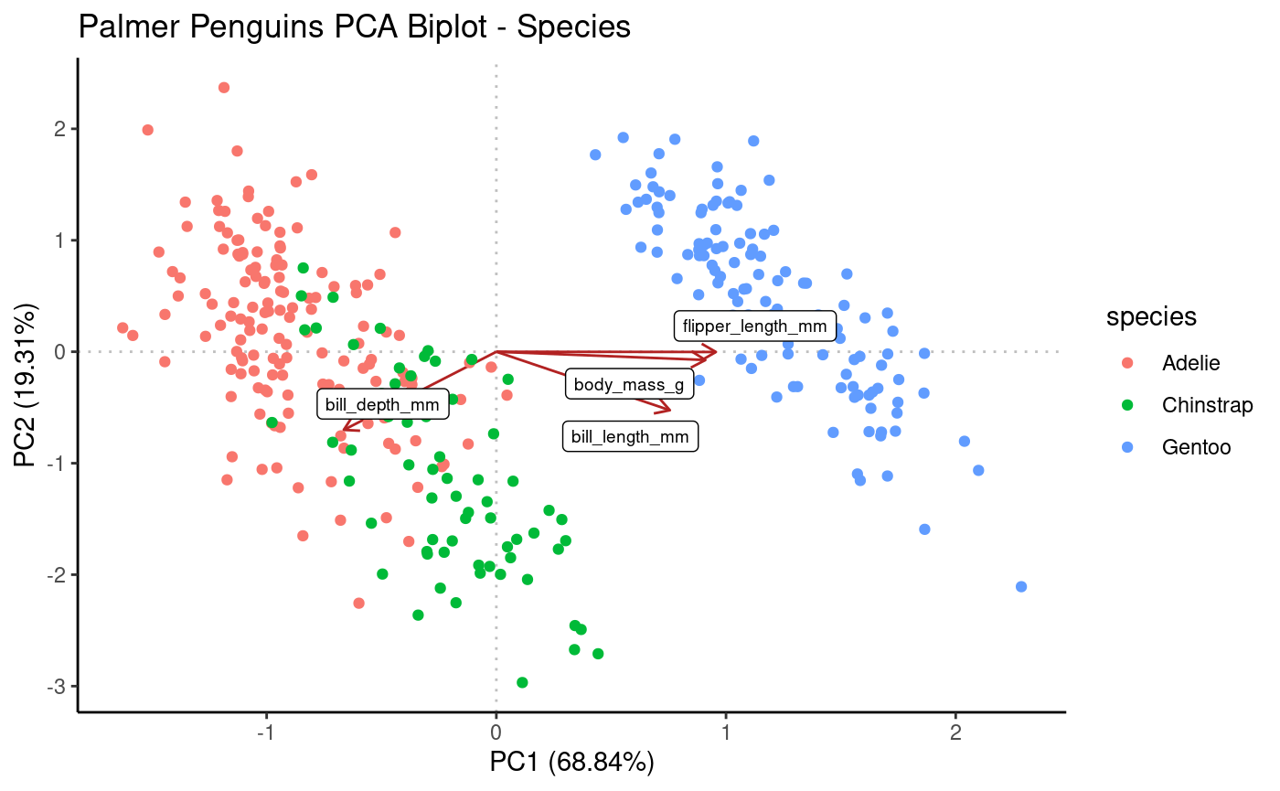
Plotting as biplot to view both (standardized) PCs and loadings on same plot.

Rubrary::plot_PCA_biplot(
  obj = pca,
  anno = penguins,
  annoname = "Sample_ID",
  annotype = "species",
  title = "Palmer Penguins PCA Biplot - Species",
  label = "Loadings"
)

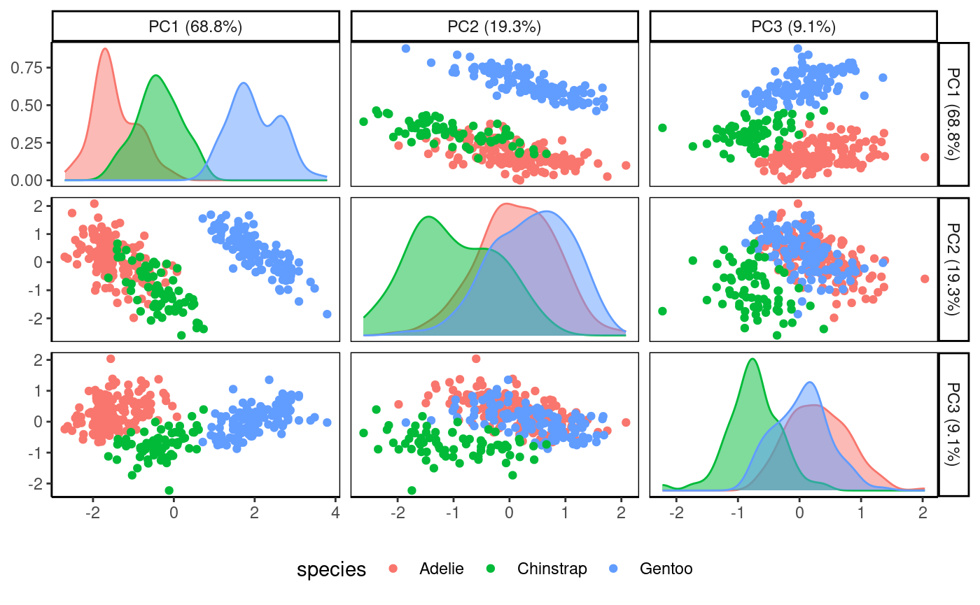
Plot multiple PCs simultaneously.

Rubrary::plot_PCA_matrix(
  df_pca = pca,
  PCs = c(1:3),
  anno = penguins,
  annoname = "Sample_ID",
  annotype = "species",
)

3D view of the first three PCs.

Rubrary::plot_PCA_3D(
  df_pca = pca,
  PCs = c(1:3),
  anno = penguins,
  annoname = "Sample_ID",
  annotype = "species",
)

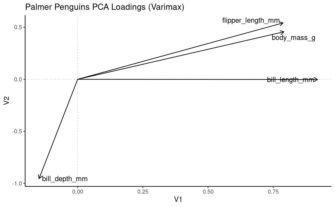
Varimax rotation

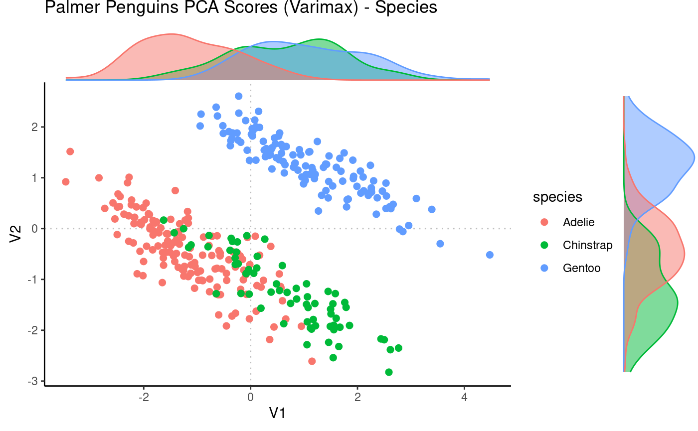
pca_vm <- Rubrary::rotate_varimax(pca)

# Visualize loadings
Rubrary::plot_PCA(
  df_pca = pca_vm$loadings,
  PCx = "V1", PCy = "V2",
  title = "Palmer Penguins PCA Loadings (Varimax)",
  type = "Loadings",
  label = TRUE
)

# Visualize scores
Rubrary::plot_PCA(
  df_pca = pca_vm$scores,
  PCx = "V1", PCy = "V2",
  anno = penguins,
  annoname = "Sample_ID",
  annotype = "species",
  title = "Palmer Penguins PCA Scores (Varimax) - Species",
  label = FALSE,
  density = TRUE,
  type = "Scores"
)

References

Beltran, Himisha, Davide Prandi, Juan Miguel Mosquera, Matteo Benelli, Loredana Puca, Joanna Cyrta, Clarisse Marotz, et al. 2016. “Divergent Clonal Evolution of Castration-Resistant Neuroendocrine Prostate Cancer.” Nature Medicine 22 (3, 3): 298–305. https://doi.org/10.1038/nm.4045.