Plot PCA biplot

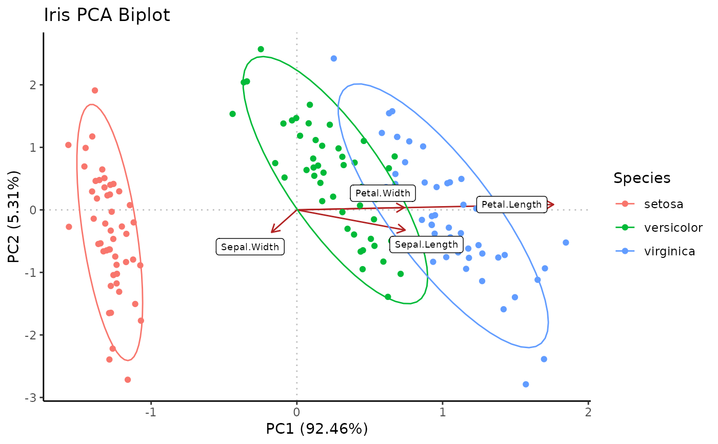
For PCA SVD \(X = USV^T\), uses standardized principal components for data points (\(\bf{U}\sqrt{n - 1}\)) and loadings (\(\bf{VS}/\sqrt{n-1}\)) and plots onto the same scale - a "proper" PCA biplot according to this Stack Exchange thread citing the Gabriel 1971 paper on PCA biplots.

Usage

plot_PCA_biplot(
  obj,
  PCx = "PC1",
  PCy = "PC2",
  anno = NULL,
  annoname = "Sample",
  annotype = "Batch",
  label = c("Both", "Loadings", "Scores", "None"),
  colors = NULL,
  col_load = "firebrick",
  title = NULL,
  ellipse = FALSE,
  savename = NULL,
  height = 8,
  width = 8
)

Arguments

obj

prcomp object

PCx

string; Component on x-axis

PCy

string; Component on y-axis

anno

df; Annotation info for observations

annoname

string; Colname in anno matching data points

annotype

string; Colname in anno for desired coloring

label

c("Both", "Loadings", "Scores", "None"); what points to label

colors

char vector; Length should be number of unique annotypes

col_load

string; Color for loading arrow segments

title

string; Plot title

ellipse

logical; Draw ggplot2::stat_ellipse data ellipse w/ default params - this is NOT a confidence ellipse

savename

string; File path to save plot under

height

numeric; Saved plot height

width

numeric; Saved plot width

Value

Biplot as ggplot object

Examples

data(iris)
iris$Sample = rownames(iris)
PCA_iris <- Rubrary::run_PCA(t(iris[,c(1:4)]),
  center = TRUE, scale = FALSE, screeplot = FALSE)
Rubrary::plot_PCA_biplot(
  obj = PCA_iris,
  anno = iris[,c("Sample", "Species")],
  annoname = "Sample", annotype = "Species",
  label = "Loadings", ellipse = TRUE, title = "Iris PCA Biplot")